UTM coordinates

Adapted from an original article by Mario Labelle

The Clubs catalogues contain UTM coordinates. These coordinates can be used to locate points on many topographical maps as, for example, the French IGN maps at 1:25000 scale (TOP25). Below, we explain what UTM coordinates are and how they can be used on the appropriate maps.

First, a little theory…

UTM stands for Universal Transverse Mercator, a cartographic projection system that divides the globe into 60 zones of 6 degrees of longitude each. Each zone is also divided at the equator into a north zone and a south zone. For example, Europe lies in zones 29-38 or, more precisely, zones north 29-38. Within each zone, any point is defined by an easting (x) and a northing (y) coordinate, expressed in metres. The coordinate is a positive number taken from the intersection of the equator and the zone’s central meridian (ie. its centre line). The values of the x coordinates range from 167000m in the west (left of the meridian) to 833 000m in the east (to the right of the meridian). The minimum is 3 degrees west of the meridian and the maximum is 3 degrees east of the meridian. In the northern hemisphere, the northing is defined simply as the distance in metres from the equator. In the southern hemisphere, to avoid negative values, 100 000 000m are added. This is, to the nearest few kilometres, the distance to the equator from the south pole. The northing always increases towards the north, that is, on maps where north is at the top. It is worth noting in passing that the Gauss-Kruger coordinates used, for example, in Germany are defined in a similar way to UTM, but with 3 degree wide zones.

Unlike coordinates of longitude and latitude that are expressed in degrees, UTM coordinates allow a direct calculation of distances between points, even if a little precision is lost as we get farther from the central meridian. However, this calculation cannot be done between points in different zones. UTM coordinates can be calculated from longitude and latitude by an approximation calculation, with an accuracy of a centimetre. The reverse calculation is also possible, but is more complicated. In any case, we must be careful to work in the same geodesic system for each system of coordinates. (WGS84 is the most commonly used geodesic system, notably for GPS).

The UTM notation varies according to which maps and applications it is used for, particularly the zone notation. The zone is sometimes omitted, sometimes only the zone is given and the hemisphere (north or south) omitted. Or the zone may be shown next to the X coordinate, either in the same font, or in a different one. The clearest way to express a point is with 3 distinct variables: zone/x/y. Here are a few examples for the same single point:
31474123 / 4769456
³¹474123 / 4769456
31 474 123 / 4 769 456
31N / 474 123 / 4 769 456

… and now in practice

For locating points on maps with metric coordinates like UTM, grid squares, usually dimensioned in kilometres, are used. This is usually noted on the map’s margins, but there may be several indications here and we must take care to use the appropriate one. For example, on French IGN TOP25 maps, UTM coordinates are in blue italics, and the grid lines are also blue.

To locate a point, we start by separating the kilometres from the metres in the UTM coordinates. Here is the example of the Col du Lourron as given in the Club’s catalogue of French cols (the ‘Chauvot’).

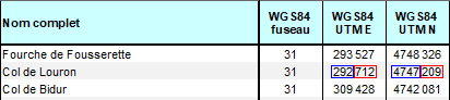
The numbers outlined in blue define the kilometre grid square to look at on the map. The numbers outlined in red indicate the position of the point in the square, in metres from its left hand side and bottom side.

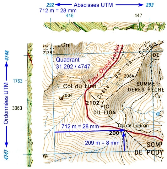
A little mental arithmetic will locate the point in the square. The red numbers are metres i.e. 1/1000s of the grid dimension, if it is 1 km. So we can see approximately where the point is. In our example, the col is shown on the TOP25 map and we easily find it at approximately 7/10 from the left and 2/10 from the bottom. For a point that isn’t marked on the map, a little sum is necessary. This is where the scale of the map (1:25000 in our case) comes into play. By dividing the metres (outlined in red) by 25, we get the millimetres on the map to measure. To divide by 25, it is an easy matter to divide by 100 and multiply by 4:

• x coordinate: 712 / 100 ~ 7, et 7 x 4 = 28 mm
• y coordinate: 209 / 100 ~ 2, et 2 x 4 = 8 mm

With a ruler, we measure 28mm from the left of the square and 4mm from the base of the square, and there you are!

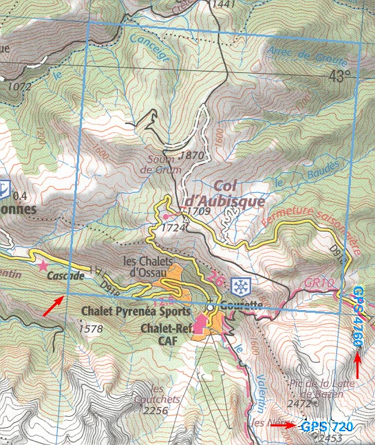
The preceding can, in principle, be used for all maps with kilometre grids. Here is a method of locating cols using coordinates from the Chauvot and IGN’s TOP100 maps.
For these, the Chauvot gives millimetre coordinates based on the TOP100 grid, making all calculation superfluous. Here, for example, shown in blue, is the grid square 715/4760 on the TOP100 map no.166. The column TOP100 in the Chauvot gives, for the Col d’Aubisque, the reference 715-4760-20-17, which places the col at 20mm from the left hand side of the square, and 17mm from its base. Note that the grid squares are 5km x 5km and we ignore the black grid lines.